# define column numbers for pattern and weight determination
col_Z2 <- which(colnames(mock_cohort) %in% "Z2")
col_U <- which(colnames(mock_cohort) %in% "U")

# define missingness pattern
default_pattern <- rep(1, ncol(mock_cohort))
pattern <- replace(default_pattern, col_Z2, 0)

# define weights
default_weights <- rep(0, ncol(mock_cohort))
weights <- replace(default_weights, c(col_Z2, col_U), c(0.2, 0.8))

prop <- 0.53 Simple de novo simulation
Simulation of different simple scenarios and missingness mitigation approaches
3.1 Objective
In this section, we will generate 1000 following different missingness scenarios.
3.2 Continuous distribution probabilities
Probabilities are based on a continuous distribution.
tic(msg = "Simulation based on continuous distribution")

results <- parallel::mclapply(
  X = 1:n_replicates,
  FUN = run_simulation,
  pattern = pattern,
  weights = weights,
  type = "RIGHT",
  prop = prop,
  mc.cores = parallel::detectCores()-1
  )

results_cont <- do.call(rbind, results) |>
  mutate(simulation = "Continuous distribution (RIGHT)")

toc()
Simulation based on continuous distribution: 1410.097 sec elapsed3.3 Discrete distribution probabilities
Probabilities are based on a discrete distribution.
tic(msg = "Simulation based on discrete distribution")

odds <- c(1, 2, 3, 4)

results <- parallel::mclapply(
  X = 1:n_replicates,
  FUN = run_simulation,
  pattern = pattern,
  weights = weights,
  odds = odds,
  prop = prop,
  mc.cores = parallel::detectCores()-1
  )

results_odds <- do.call(rbind, results) |>
  mutate(simulation = paste0("Discrete odds (", paste0(odds, collapse = ", "), ")"))

toc()
Simulation based on discrete distribution: 1381.326 sec elapsed3.4 Save simulation results
results <- rbind(results_cont, results_odds) |>
  mutate(method = factor(method, levels = c(
    "Unadjusted",
    "Complete case",
    "Imputed"))
    )
3.5 Results
The next steps of this script analyze the raw simulation results obtained in the previous script via run_simulation.R. The last run on 2024-11-01 18:20:43.222866.
3.6 Read raw results table
We first look at the results table with the raw simulation results.
results |>
  glimpse()
Rows: 6,000
Columns: 5
$ method <fct> Unadjusted, Complete case, Imputed, Unadjusted, Complete ca…
$ estimate <dbl> 1.2629630, 0.8932111, 0.9111699, 1.1150121, 0.8824297, 1.03…
$ se <dbl> 0.07923421, 0.13274238, 0.10924959, 0.07479571, 0.11677905,…
$ replicate <int> 1, 1, 1, 2, 2, 2, 3, 3, 3, 4, 4, 4, 5, 5, 5, 6, 6, 6, 7, 7,…
$ simulation <chr> "Continuous distribution (RIGHT)", "Continuous distribution…3.7 QC
Let’s do a few quality/sanity checks.
- Number of analysis methods
unique(results$method)[1] Unadjusted Complete case Imputed
Levels: Unadjusted Complete case Imputed- Assert that there are no missing results
assert_that(!any(sapply(results$estimate, is.na)), msg = "There are missing estimates")[1] TRUEassert_that(!any(sapply(results$se, is.na)), msg = "There are missing standard errors")[1] TRUE3.8 Main results
# call helper functions
source(here::here("functions", "rsimsum_ggplot.R"))
For the analysis of aggregate simulation results we use the rsimsum package. More information about this package can be found here.[@rsimsum]
simsum_out <- simsum(
  data = results,
  estvarname = "estimate",
  se = "se",
  true = 1,
  by = "simulation",
  methodvar = "method",
  ref = "Complete case"
  ) |>
  summary() |>
tidy()hr_distribution <- results |>
ggplot(aes(x = method, y = estimate)) +
geom_boxplot(outlier.colour = "red") +
geom_point(position = position_jitter(seed = 42), alpha = 0.15) +
geom_hline(yintercept = 1.0, color = "forestgreen", linetype = "dashed") +
labs(
x = "Method",
y = "Hazard ratio (HR)"
) +
theme_bw() +
theme(
axis.title.x = element_blank(),
axis.text.x = element_text(angle = 35, vjust = 1, hjust=1)
) +
facet_wrap(~simulation)
hr_distribution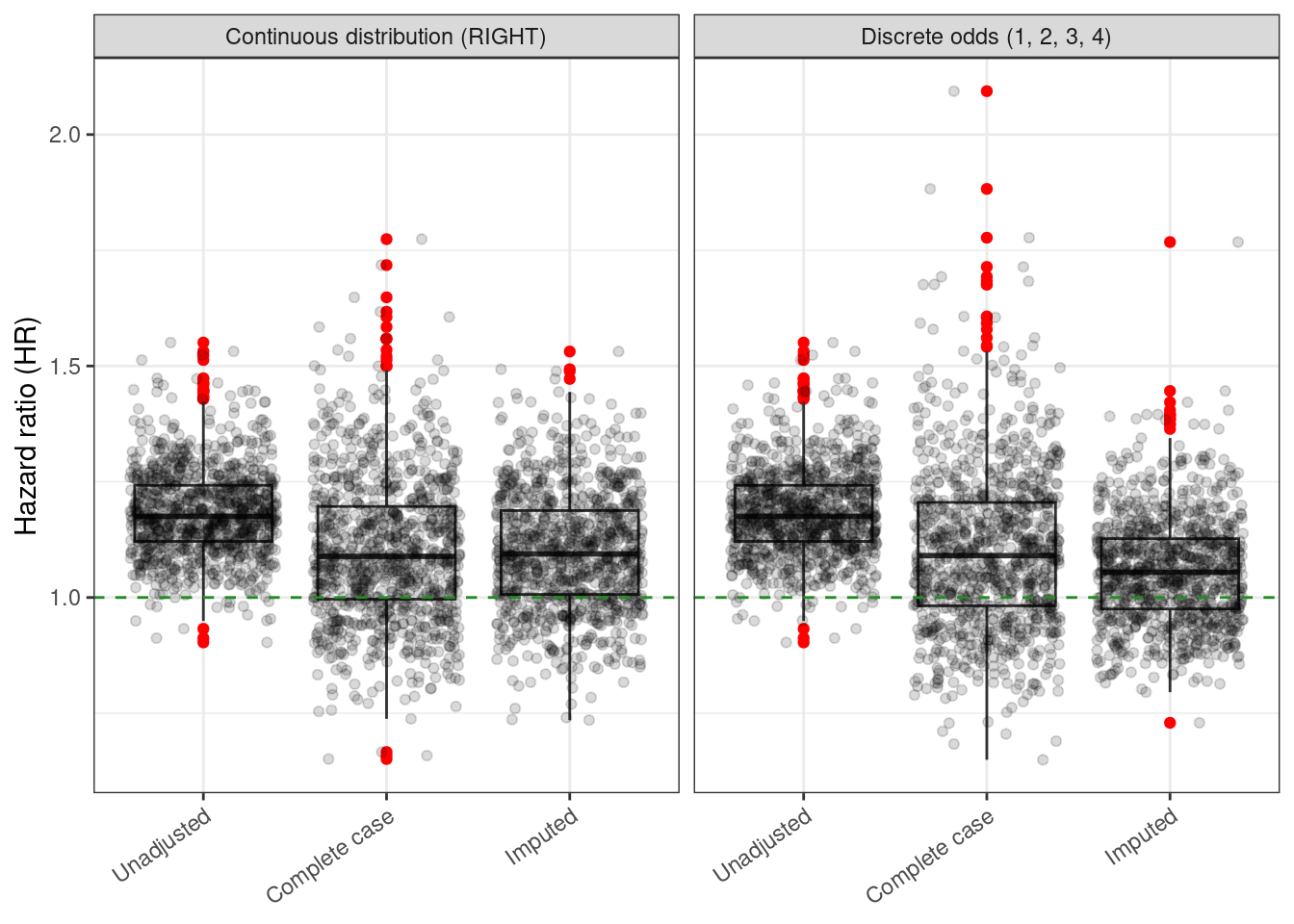
ggplotly(hr_distribution)3.8.1 Root mean squared error (RMSE)
rmse <- rsimsum_ggplot(tidy_simsum = simsum_out, metric = "rmse")rmse$plot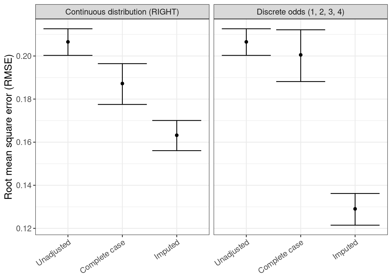
rmse$table |>
gt()| method | est | lower | upper |
|---|---|---|---|
| Continuous distribution (RIGHT) | |||
| Unadjusted | 0.207 | 0.200 | 0.213 |
| Complete case | 0.187 | 0.178 | 0.196 |
| Imputed | 0.163 | 0.156 | 0.170 |
| Discrete odds (1, 2, 3, 4) | |||
| Unadjusted | 0.207 | 0.200 | 0.213 |
| Complete case | 0.201 | 0.188 | 0.212 |
| Imputed | 0.129 | 0.121 | 0.136 |
3.8.2 Bias
bias <- rsimsum_ggplot(tidy_simsum = simsum_out, metric = "bias")bias$plot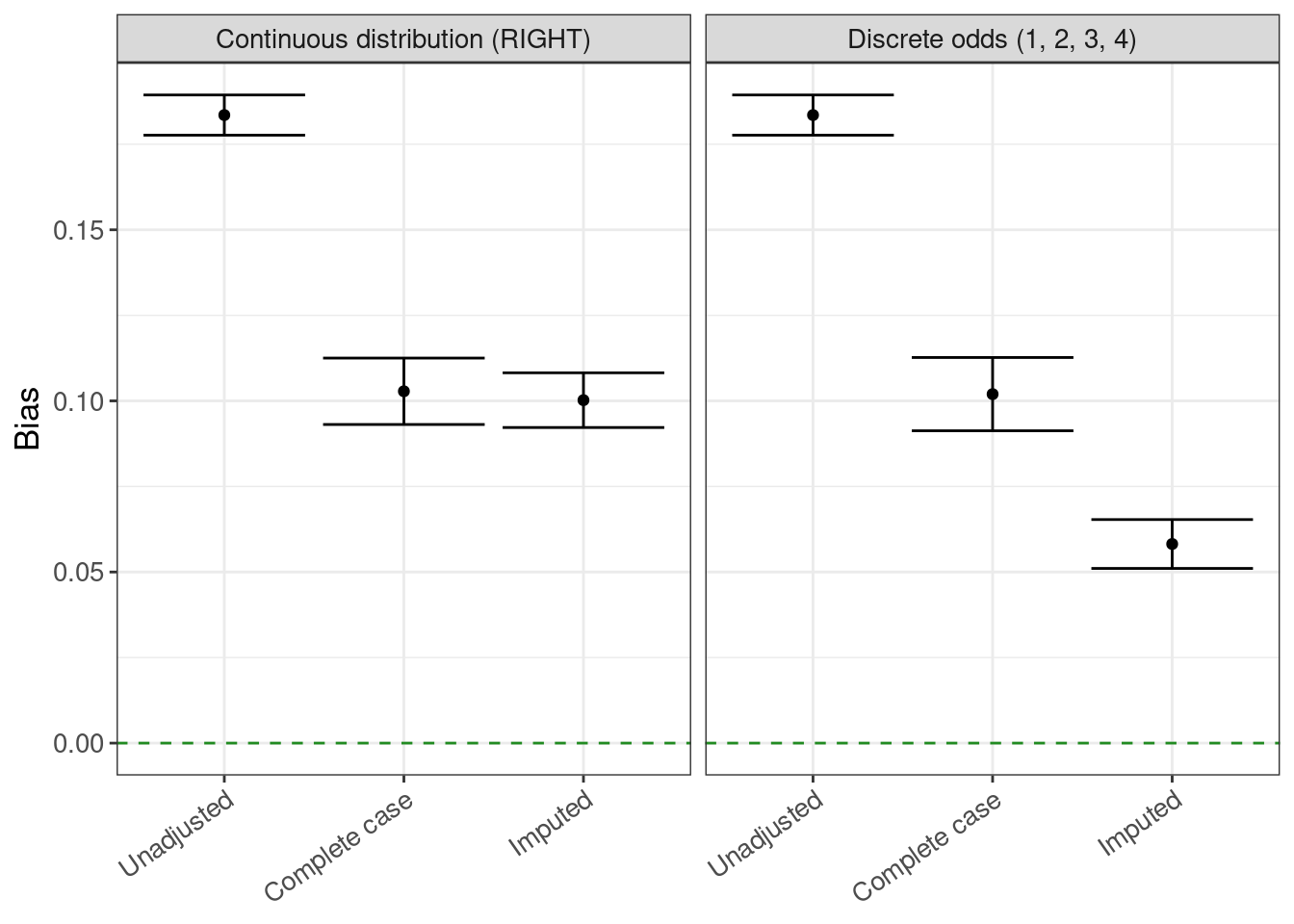
bias$table |>
gt()| method | est | lower | upper |
|---|---|---|---|
| Continuous distribution (RIGHT) | |||
| Unadjusted | 0.184 | 0.178 | 0.189 |
| Complete case | 0.103 | 0.093 | 0.113 |
| Imputed | 0.100 | 0.092 | 0.108 |
| Discrete odds (1, 2, 3, 4) | |||
| Unadjusted | 0.184 | 0.178 | 0.189 |
| Complete case | 0.102 | 0.091 | 0.113 |
| Imputed | 0.058 | 0.051 | 0.065 |
3.8.3 Coverage
coverage <- rsimsum_ggplot(tidy_simsum = simsum_out, metric = "coverage")coverage$plot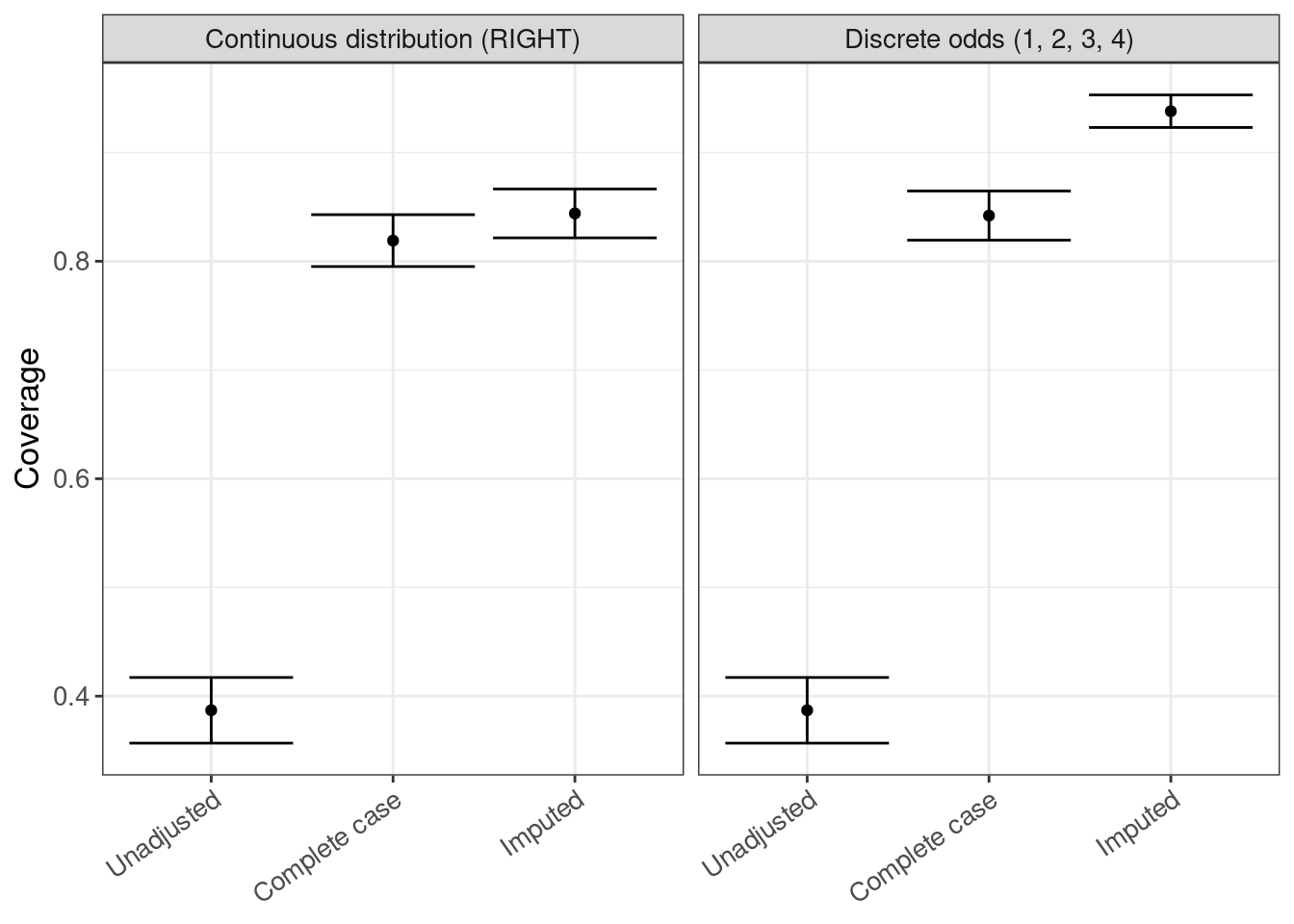
coverage$table |>
gt()| method | est | lower | upper |
|---|---|---|---|
| Continuous distribution (RIGHT) | |||
| Unadjusted | 0.387 | 0.357 | 0.417 |
| Complete case | 0.819 | 0.795 | 0.843 |
| Imputed | 0.844 | 0.822 | 0.866 |
| Discrete odds (1, 2, 3, 4) | |||
| Unadjusted | 0.387 | 0.357 | 0.417 |
| Complete case | 0.842 | 0.819 | 0.865 |
| Imputed | 0.938 | 0.923 | 0.953 |
3.8.4 Empirical standard error
empse <- rsimsum_ggplot(tidy_simsum = simsum_out, metric = "empse")empse$plot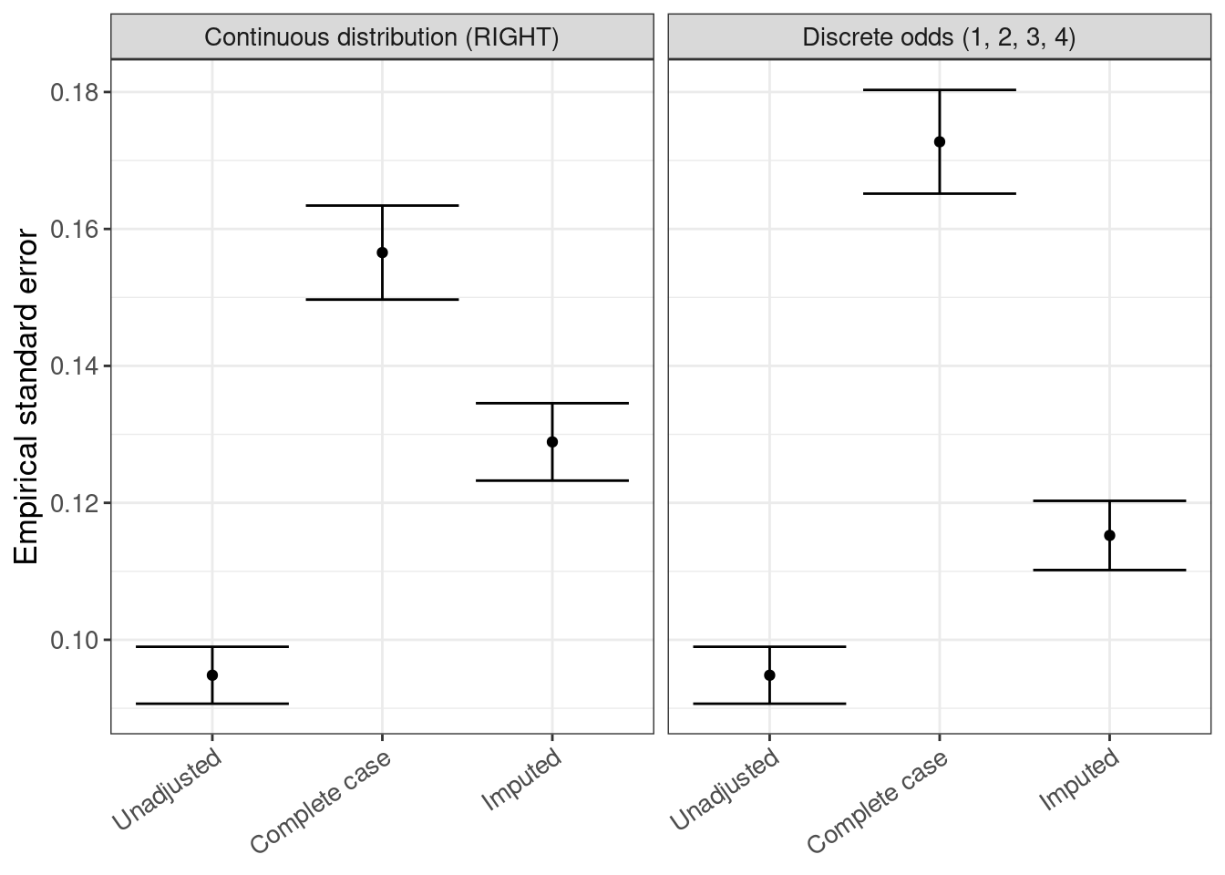
empse$table |>
gt()| method | est | lower | upper |
|---|---|---|---|
| Continuous distribution (RIGHT) | |||
| Unadjusted | 0.095 | 0.091 | 0.099 |
| Complete case | 0.157 | 0.150 | 0.163 |
| Imputed | 0.129 | 0.123 | 0.135 |
| Discrete odds (1, 2, 3, 4) | |||
| Unadjusted | 0.095 | 0.091 | 0.099 |
| Complete case | 0.173 | 0.165 | 0.180 |
| Imputed | 0.115 | 0.110 | 0.120 |
3.9 Session info
Total script runtime: 46.57 minutes.
pander::pander(subset(data.frame(sessioninfo::package_info()), attached==TRUE, c(package, loadedversion)))| package | loadedversion | |
|---|---|---|
| assertthat | assertthat | 0.2.1 |
| dplyr | dplyr | 1.1.4 |
| ggplot2 | ggplot2 | 3.4.4 |
| gt | gt | 0.10.1 |
| here | here | 1.0.1 |
| plotly | plotly | 4.10.4 |
| rsimsum | rsimsum | 0.11.3 |
| tictoc | tictoc | 1.2 |
| tidyr | tidyr | 1.3.1 |
pander::pander(sessionInfo())R version 4.4.0 (2024-04-24)
Platform: x86_64-pc-linux-gnu
locale: LC_CTYPE=C.UTF-8, LC_NUMERIC=C, LC_TIME=C.UTF-8, LC_COLLATE=C.UTF-8, LC_MONETARY=C.UTF-8, LC_MESSAGES=C.UTF-8, LC_PAPER=C.UTF-8, LC_NAME=C, LC_ADDRESS=C, LC_TELEPHONE=C, LC_MEASUREMENT=C.UTF-8 and LC_IDENTIFICATION=C
attached base packages: parallel, stats, graphics, grDevices, datasets, utils, methods and base
other attached packages: plotly(v.4.10.4), tidyr(v.1.3.1), assertthat(v.0.2.1), rsimsum(v.0.11.3), gt(v.0.10.1), ggplot2(v.3.4.4), tictoc(v.1.2), dplyr(v.1.1.4) and here(v.1.0.1)
loaded via a namespace (and not attached): sass(v.0.4.8), utf8(v.1.2.4), generics(v.0.1.3), renv(v.1.0.3), xml2(v.1.3.6), digest(v.0.6.33), magrittr(v.2.0.3), evaluate(v.0.23), grid(v.4.4.0), fastmap(v.1.1.1), rprojroot(v.2.0.4), jsonlite(v.1.8.8), sessioninfo(v.1.2.2), backports(v.1.4.1), httr(v.1.4.7), pander(v.0.6.5), purrr(v.1.0.2), fansi(v.1.0.6), crosstalk(v.1.2.1), viridisLite(v.0.4.2), scales(v.1.3.0), lazyeval(v.0.2.2), cli(v.3.6.2), rlang(v.1.1.2), ellipsis(v.0.3.2), munsell(v.0.5.0), withr(v.3.0.0), yaml(v.2.3.8), tools(v.4.4.0), checkmate(v.2.3.1), colorspace(v.2.1-0), vctrs(v.0.6.5), R6(v.2.5.1), ggridges(v.0.5.6), lifecycle(v.1.0.4), htmlwidgets(v.1.6.4), simsurv(v.1.0.0), pkgconfig(v.2.0.3), pillar(v.1.9.0), gtable(v.0.3.4), Rcpp(v.1.0.12), glue(v.1.6.2), data.table(v.1.15.0), xfun(v.0.41), tibble(v.3.2.1), tidyselect(v.1.2.0), knitr(v.1.45), farver(v.2.1.1), htmltools(v.0.5.7), rmarkdown(v.2.28), labeling(v.0.4.3) and compiler(v.4.4.0)
pander::pander(options('repos'))repos:
REPO_NAME https://packagemanager.posit.co/cran/latest